Set Up: To set up this problem, we were able to use the same spatial molecule from the previous problem, but this time including a time-stepping scheme.
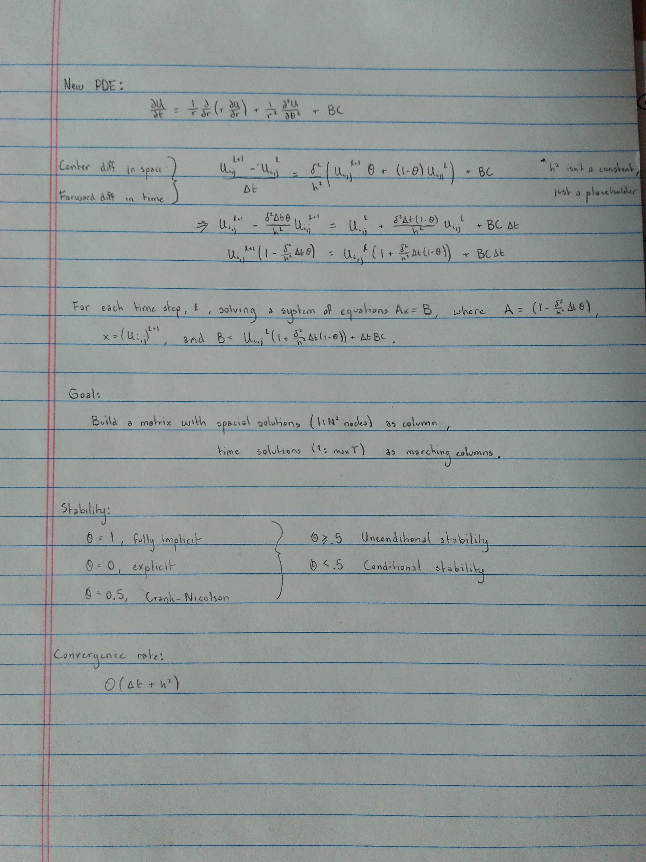
For this molecule and problem, we expect to see the truncation error go as O(k+h^2), due to forward difference in time and center difference in space.
At theta = 0.5, we have O(k^2 + h^2) - Crank-Nicolson.
Dirichlet boundary condition:
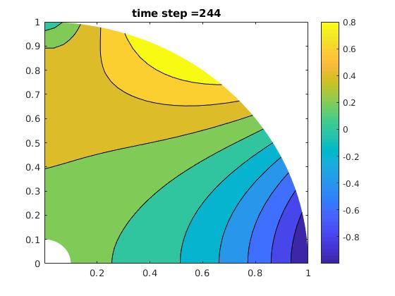
Steady-State with r=10 and theta=0.6:
Play movie.
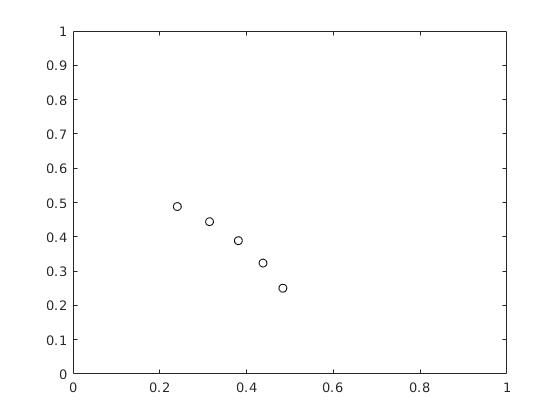
Individual Point plots:
Convergence with N=80:

Part 2:
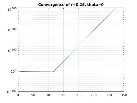
r = 0.25, theta = 0.0
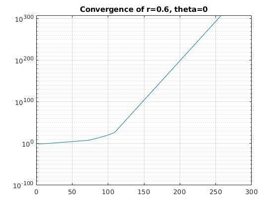
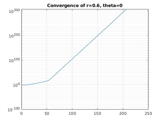
r = 0.60, theta = 0.0
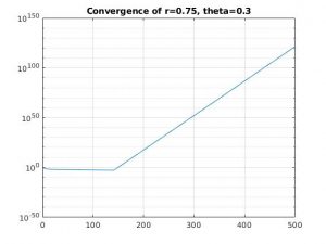
r = 0.75, theta = 0.3
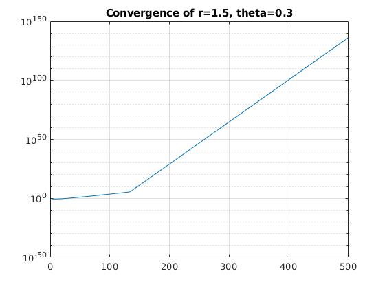
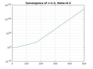
r = 1.50, theta = 0.3
r = 10.0, theta = 0.6
For each of the first four combinations of parameters, we see that the solution diverges. This is because when theta < 0.5, we have conditional stability that depends on the values of r.
For the 1D problem, we expect bounded solutions for values of r less than 0.25 when theta is 0. When theta is 0.3, we need values of r less than .357, which we don't have. When theta is greater than 0.5, we have unconditional stability and the values of r are inconsequential.
Part 3:
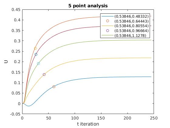
We can estimate the time constant for the solution by finding the steady-state value, U_f, and then multiplying by 1-1/e. Then we find the time iteration, t, that corresponds to the value, and multiply by ∆t to get the time constants.
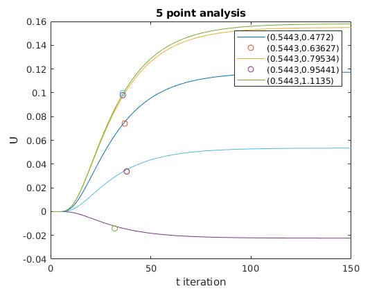
As we can see from the graph, all 5 points in the interior of the geometry showing converging behavior. For each of the 5 points, we get time constants that are very close to each other.
time constants = [ 0.0415, 0.0493, 0.0480, 0.0467, 0.0467]
ROBIN Boundary Condition:
Steady-State with r=10 and theta=0.6:
Play movie.
Part 2:
r = 0.25, theta = 0.0

r = 0.60, theta = 0.0
r = 0.75, theta = 0.3

r = 1.50, theta = 0.3
r = 10.0, theta = 0.6
Part 3:
We can estimate the time constant for the solution by finding the steady-state value, U_f, and then multiplying by 1-1/e. Then we find the time iteration, t, that corresponds to the value, and multiply by ∆t to get the time constants.
As we can see from the graph, all 5 points in the interior of the geometry showing converging behavior. For each of the 5 points, we get time constants that are less similar than before.
time constants = [ 0.3195, 0.2237, 0.1651, 0.1385, 0.1331 ]