Part A:
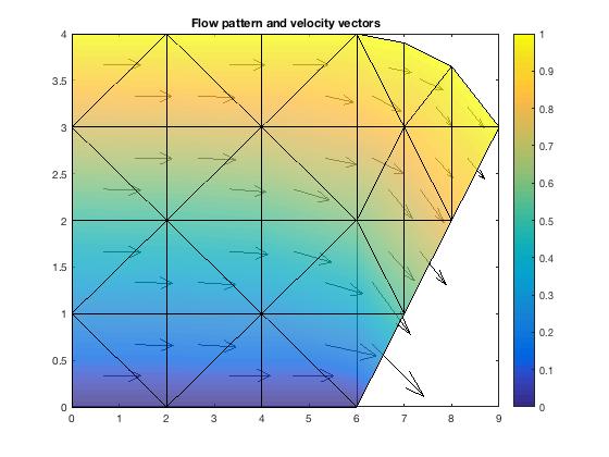
In the first part of the problem, we have a 38 elements and 28 nodes to consider for the FEM analysis. Using the given boundary conditions and symmetry argument, we can simulate the flow pattern through a rectangular ventilating duct.
Following the example in Chapter 9 of the textbook, I was able to build the A matrix and boundary condition vector using Fortran, and solve the equation Ax = b using the DSOLVE subroutine. After exporting the data into Matlab, the final simulation is presented below.
Part B:
The only change in this section is to change the boundary condition of the symmetry axis. Instead of having a homogeneous flux condition, we now have one more node with a condition psi = 1.

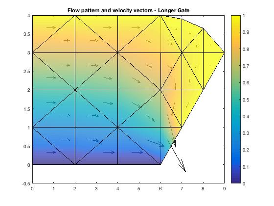
Part C:
The gate is extended one node further for this part of the problem.
Code:
program HW3
implicit none
integer :: NH, n1, n2, n3, i,j, x_nod, y_nod, elem(38,4), D_top(9), D_bot(4), D_lef(3)
real*8 :: x1, x2, x3, y1, y2, y3, area, x_cent, y_cent, node(28,3)
real*8 :: A_e(3,3), A(28,28), B(28), A_band(28,11), vel_x(38), vel_y(38), x_centers(38), y_centers(38)
! load in elem and node matrices
open( unit=9, file='hw5.nodes.dat', status='unknown')
do i = 1,28
read(9,*) (node(i,j), j=1,3) ! put in values of node points
end do
close(9)
open( unit=10, file='hw5.elems.dat', status='unknown')
do i = 1,38
read(10,*) (elem(i,j), j=1,4)
end do
close(10)
! zero out A and A_e
A = 0.d0
A_e = 0.d0
! do loop through element file
do i = 1,38
n1 = elem(i,2)
n2 = elem(i,3)
n3 = elem(i,4)
! assign coordinates to each node in current element
x1 = node(n1,2)
y1 = node(n1,3)
x2 = node(n2,2)
y2 = node(n2,3)
x3 = node(n3,2)
y3 = node(n3,3)
! compute area of current element
area = (x1*(y2-y3) + x2*(y3-y1) + x3*(y1-y2)) / 2
A_e(1,1) = -(((y2-y3)*(y2-y3))+((x2-x3)*(x2-x3))) / (4*area)
A_e(1,2) = -(((y2-y3)*(y3-y1))+((x2-x3)*(x3-x1))) / (4*area)
A_e(1,3) = -(((y2-y3)*(y1-y2))+((x2-x3)*(x1-x2))) / (4*area)
A_e(2,1) = -(((y3-y1)*(y2-y3))+((x3-x1)*(x2-x3))) / (4*area)
A_e(2,2) = -(((y3-y1)*(y3-y1))+((x3-x1)*(x3-x1))) / (4*area)
A_e(2,3) = -(((y3-y1)*(y1-y2))+((x3-x1)*(x1-x2))) / (4*area)
A_e(3,1) = -(((y1-y2)*(y2-y3))+((x1-x2)*(x2-x3))) / (4*area)
A_e(3,2) = -(((y1-y2)*(y3-y1))+((x1-x2)*(x3-x1))) / (4*area)
A_e(3,3) = -(((y1-y2)*(y1-y2))+((x1-x2)*(x1-x2))) / (4*area)
! put into global matrix A
A(n1,n1) = A(n1,n1) + A_e(1,1)
A(n1,n2) = A(n1,n2) + A_e(1,2)
A(n1,n3) = A(n1,n3) + A_e(1,3)
A(n2,n1) = A(n2,n1) + A_e(2,1)
A(n2,n2) = A(n2,n2) + A_e(2,2)
A(n2,n3) = A(n2,n3) + A_e(2,3)
A(n3,n1) = A(n3,n1) + A_e(3,1)
A(n3,n2) = A(n3,n2) + A_e(3,2)
A(n3,n3) = A(n3,n3) + A_e(3,3)
enddo
! boundary conditions
! dirichlet nodes
D_top = [5,10,15,20,21,24,25,27,28] ! = 1
D_bot = [1,6,11,16] ! = 0
D_lef = [2,3,4] ! = y/L
! neuman nodes
! (16,21,25,28) => dU/dn = 0
B = 0.d0
do i=1,28
do j=1,9
if (node(i,1) == D_top(j)) then
B(i) = 1
A(i,:) = 0
A(i,i) = 1
endif
enddo
do j=1,4
if (node(i,1) == D_bot(j)) then
B(i) = 0
A(i,:) = 0
A(i,i) = 1
endif
enddo
do j=1,3
if (node(i,1) == D_lef(j)) then
B(i) = node(i,3)/4.
A(i,:) = 0
A(i,i) = 1
endif
enddo
enddo
!open( unit=11, file='BC.dat')
!open( unit=12, file='A_mat.dat')
!do i=1,28
! write(11,*), B(i)
! write(12,*), (A(i,j), j=1,28)
!enddo
!close(11)
!close(12)
NH = 5
! band A matrix for solver
do i=1,28
do j=1,28
if (A(i,j).ne.0.) then
A_band(i,(NH+1)+(j-i)) = A(i,j)
endif
enddo
enddo
CALL DSOLVE( 3, A_band, B, 28, NH, 28, 2*NH+1)
open(unit=13, file='sol_c.dat')
do i=1,28
write(13,*), B(i)
enddo
close(13)
! compute x and y velocities
do i = 1,38
n1 = elem(i,2)
n2 = elem(i,3)
n3 = elem(i,4)
! assign coordinates to each node in current element
x1 = node(n1,2)
y1 = node(n1,3)
x2 = node(n2,2)
y2 = node(n2,3)
x3 = node(n3,2)
y3 = node(n3,3)
! compute area of current element
area = (x1*(y2-y3) + x2*(y3-y1) + x3*(y1-y2)) / 2
vel_x(i) = B(n1)*(y2-y3)/(2*area) + B(n2)*(y3-y1)/(2*area) + B(n3)*(y1-y2)/(2*area)
vel_y(i) = -( B(n1)*(x2-x3)/(2*area) + B(n2)*(x3-x1)/(2*area) + B(n3)*(x1-x2)/(2*area) )
x_centers(i) = (x1+x2+x3)/3.
y_centers(i) = (y1+y2+y3)/3.
enddo
open(unit=14, file='x_cent_c.dat')
open(unit=15, file='y_cent_c.dat')
open(unit=16, file='x_vel_c.dat')
open(unit=17, file='y_vel_c.dat')
do i = 1,38
write(14,*), x_centers(i)
write(15,*), y_centers(i)
write(16,*), vel_x(i)
write(17,*), vel_y(i)
enddo
close(14)
close(15)
close(16)
close(17)
end program HW3
! SYSTEM FORTRAN-90
! LAST MODIFICATION BY Matt McGarry, 13 jan2012 - Changed to F90 format
!------------------------------------------------------------
! B = LHS MATRIX , DIMENSIONED (NDIM,MDIM) IN CALLING PROGRAM
! R = RIGHT-HAND-SIDE, DIMENSIONED (NDIM) IN CALLING PROGRAM
! NEQ= # OF EQUATIONS
! IHALFB= HALF-BANDWIDTH; 2*IHALFB+1 = BANDWIDTH
! SOLUTION RETURNS IN R
! KKK = 1 PERFORMS LU DECOMPOSITION DESTRUCTIVELY
! KKK = 2 PERFORMS BACK SUBSTITUTION
! KKK = 3 PERFORMS OPTIONS 1 AND 2
!
SUBROUTINE DSOLVE(KKK,B,R,NEQ,IHALFB,NDIM,MDIM)
!
! ASYMMETRIC BAND MATRIX EQUATION SOLVER (DOUBLE PRECISION)
! DOCTORED TO IGNORE ZEROS IN LU DECOMP. STEP
!
INTEGER KKK,NEQ,IHALFB,NDIM,MDIM
REAL*8 B(NDIM,MDIM),R(NDIM)
NRS=NEQ-1
IHBP=IHALFB+1
IF (KKK.EQ.2) GO TO 30
!
! TRIANGULARIZE MATRIX A USING DOOLITTLE METHOD
!
DO 10 K=1,NRS
PIVOT=B(K,IHBP)
KK=K+1
KC=IHBP
DO 21 I=KK,NEQ
KC=KC-1
IF(KC.LE.0) GO TO 10
C=-B(I,KC)/PIVOT
IF (C.EQ.0.D0) GO TO 21
B(I,KC)=C
KI=KC+1
LIM=KC+IHALFB
DO 20 J=KI,LIM
JC=IHBP+J-KC
20 B(I,J)=B(I,J)+C*B(K,JC)
21 CONTINUE
10 CONTINUE
IF(KKK.EQ.1) GO TO 100
!
! MODIFY LOAD VECTOR R
!
30 NN=NEQ+1
IBAND=2*IHALFB+1
DO 40 I=2,NEQ
JC=IHBP-I+1
JI=1
IF (JC.LE.0) GO TO 50
GO TO 60
50 JC=1
JI=I-IHBP+1
60 SUM=0.0
DO 70 J=JC,IHALFB
SUM=SUM+B(I,J)*R(JI)
70 JI=JI+1
40 R(I)=R(I)+SUM
!
! BACK SOLUTION
!
R(NEQ)=R(NEQ)/B(NEQ,IHBP)
DO 80 IBACK=2,NEQ
I=NN-IBACK
JP=I
KR=IHBP+1
MR=MIN0(IBAND,IHALFB+IBACK)
SUM=0.0
DO 90 J=KR,MR
JP=JP+1
90 SUM=SUM+B(I,J)*R(JP)
80 R(I)=(R(I)-SUM)/B(I,IHBP)
100 RETURN
END SUBROUTINE