The major change from last week is now boundary A (theta = pi/2) has a Robin condition. I followed the same process of solving along the boundary with a ghost node. This resulted in the molecule shown in the figure below.
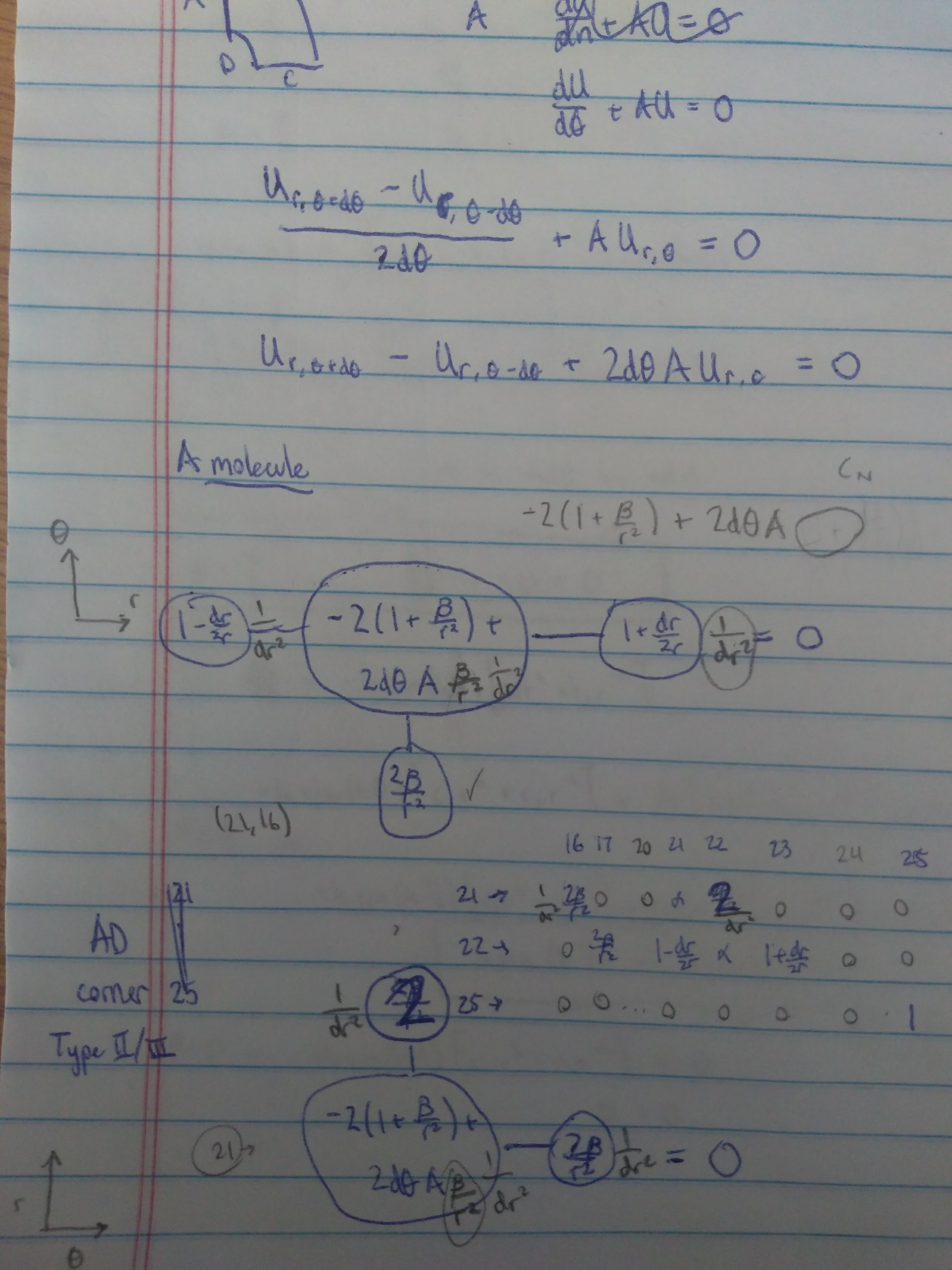
This meant that the corner between boundaries A and D had to be changed as well, since A no longer had the Dirichlet condition. The corner molecule is also shown above.
Effect of A:
For this part, I used the single precision solver Solve.f in Fortran and plotted the solutions in MATLAB. I chose 3 values of A, ranging from .01 to 10000.
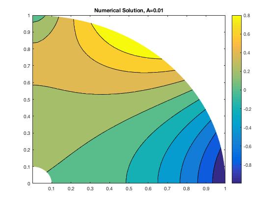
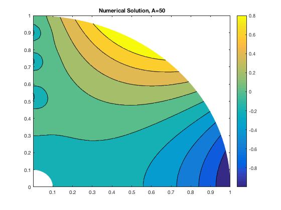
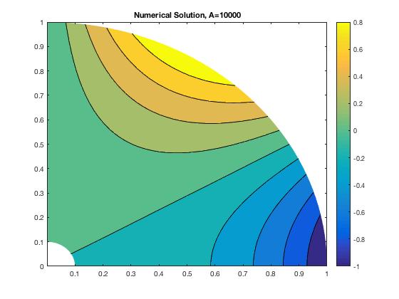
For a low value of A, the solution shows Neumann boundary condition behavior. For this boundary, we have prescribed heat flux, with A equal to the heat transfer coefficient. When A is very low, we expect to see a normal gradient condition. As A increases, the behavior becomes much more mixed until high values of A, when the boundary takes on Dirichlet behavior. Then the boundary has a prescribed temperature, which should all be 0.
Part 2: Iterative Solvers
For this section, the analytic solution is calculated using N=160 using the direct solver in Matlab.
Jacobi, Gauss-Seidel, SOR:


SOR:
For the SOR method with w=1, we get the Gauss-Seidel iteration method back. If w<1, then the iteration method would include a damping factor, but if w>1 then the Gauss-Seidel method would be 'accelerated'. The optimal choice for w is 2 / (1+ sqrt(1 - rho(GS) ). If the spectral radius from the Gauss-Seidel method is ideally almost 1, then w ≈ 1.81, which is still within the bounds of stability. For my solutions, I used w = 1.2 in order to achieve convergence.
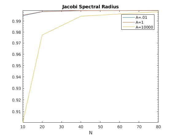
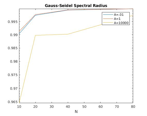
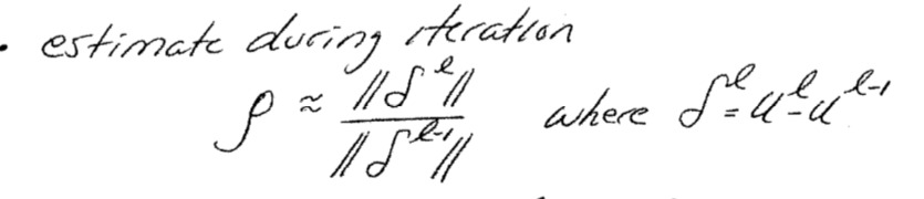
Spectral Radius:
To find the spectral radius of each iteration method, I used the formula below during each iteration, l.
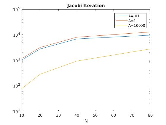
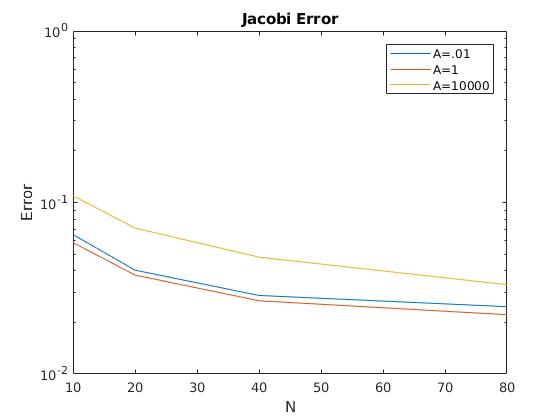
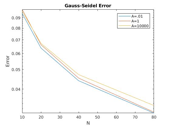
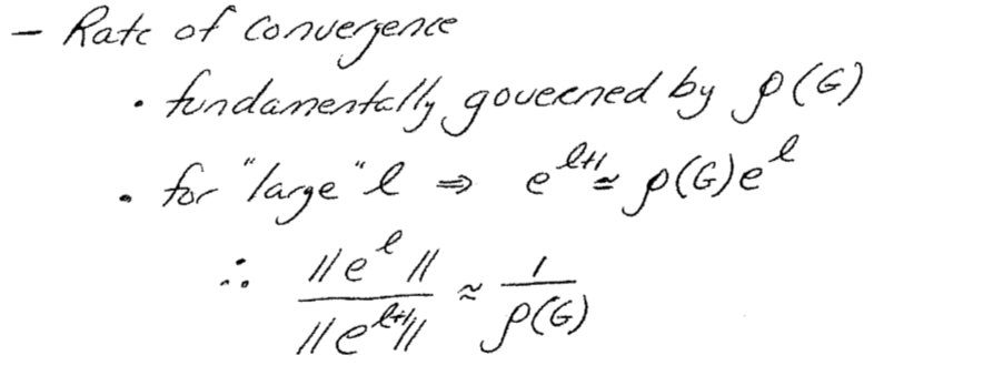
Convergence Rates:
According to theory, the Jacobi method should have a convergence rate of h^2 / 2, while Gauss-Seidel is h^2 and SOR is 2*h. All of these convergence rates can be determined by the spectral radius.
In my simulations, it's hard to draw conclusions of the solvers with only 3 N values. Both the error of the Jacobi and the Gauss-Seidel methods have similar trends, whereas for SOR, the error increases as N increases.