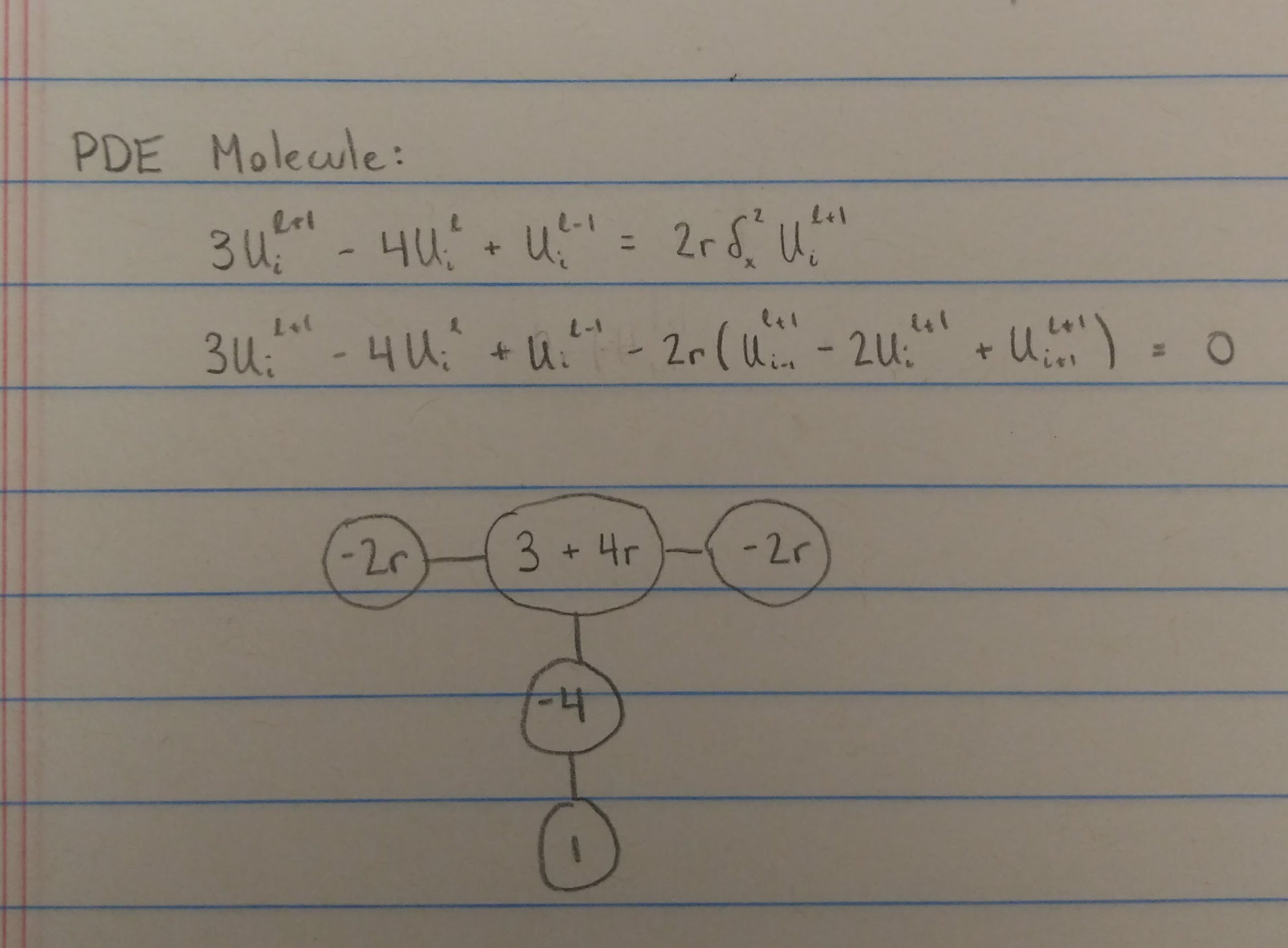
In order to investigate this FD scheme for the 1D diffusion equation, we need to consider the consistency, stability, and accuracy of the scheme. The first step is to create a molecule, which will contain 3 spatial terms and 3 time levels. Immediately, we recognize the need for two initial conditions in order for the method to get started.
Consistency:
The first step in analyzing the consistency of this FD scheme is to look for familiar terms. The spatial derivative in the diffusion equation is approximated using the second order central difference. For this, we already know the expected order of convergence and the leading truncation error term, shown below.
For the time derivative, this scheme is not immediately recognizable. But if we go back to the Taylor expansion, we can create a FD scheme for a first order derivative to O(h^2). This derivation is also shown below, along with the leading truncation error term.

Stability:
Using the Von Neumann method to analyze stability, we find restrictions on r that determine the convergence of the system.

After finding that we need r≥0 for stability, we can check how this condition holds in the numerical solution.

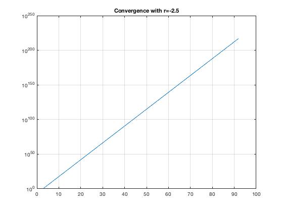
We can see that for any positive value of r, we have the expected convergence and the correct convergence rate. And for negative r, the solution diverges as soon as it starts.
Accuracy:
Continuing with the stability analysis, we can also check on the accuracy of the system. Solving for the amplification factor, gamma, we can analyze the behavior of short and long wavelengths.

For shorter wavelengths, we have an imaginary amplification factor when r > 1/8. As a result, there will be temporal oscillations of period 8∆t when -1 < gamma < 0. The oscillatory behavior reinforces the fact that shorter wavelengths will be the first to misbehave in the numerical solution.
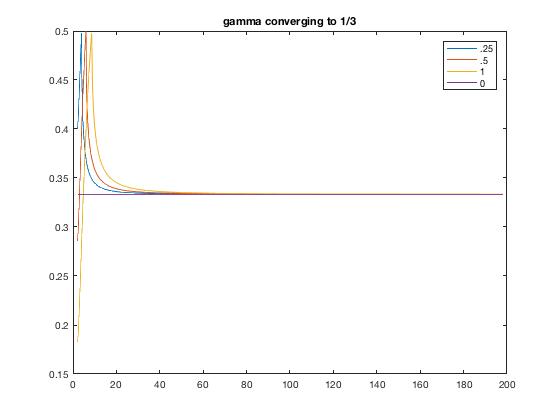
For longer wavelengths, we have two positive amplification factors, but only one is the physical solution. The first one, where gamma = 1, will propagate, whereas gamma = 1/3 is parasite.
D: Changing the spatial derivative -
For this part, we investigate how the FD scheme would work if the spatial derivative is at time level l. For consistency, the time derivative is the same as in the first part, so the order of convergence will remain the same. As for the spatial derivative, the time step does not affect the center difference, so it also has the same order of convergence.
For stability, we follow the same process as before, using Von Neumann analysis. We find the same restriction on r as before, where r has to be positive for a stable solution.
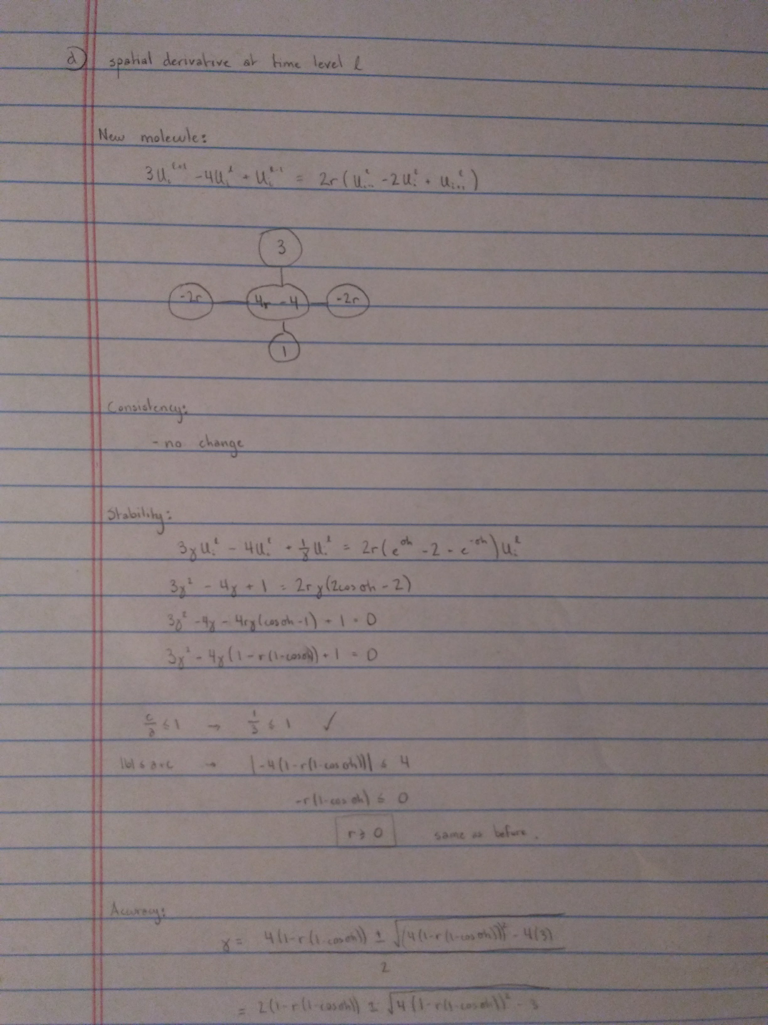
For consistency, stability, and accuracy, the new FD scheme behaves the same as the originally proposed scheme.
E: Coding -
Using only the spatial terms of the PDE molecule on a 1D geometry, and storing the solutions as a function of time. This allows for easy access of the previous time solutions in determining the current time level. Using the given boundary and initial conditions, the final solution looks like below.
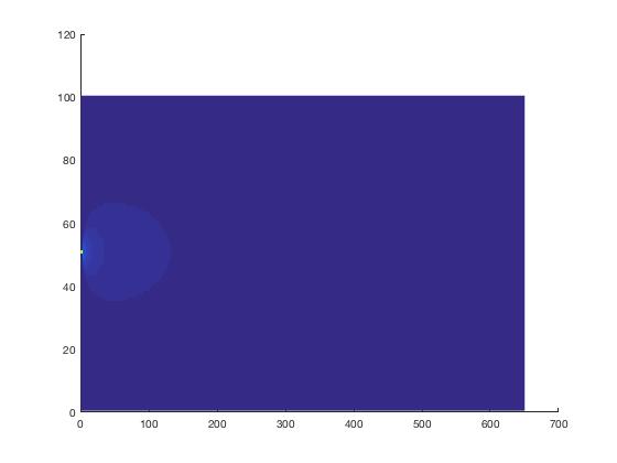
We have a gaussian distribution as the initial conditions at ∆t=0 and ∆t=-∆t, which is sufficient to start the method. As soon as the scheme begins, the diffusion can be seen in the image above until everything reaches equilibrium. The solution stops once the norm of U(x,t+∆t) reaches a tolerance of 1e-5.
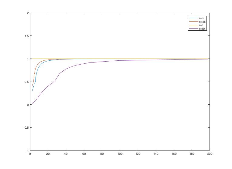
Varying the parameters shows that convergence will hold for all r values above 0, but the convergence rate changes based these values.

If we vary the spatial step size h, we can see that the convergence rate is affected by this value, but will still reach convergence. As h increases in size, then r is decreasing, which means that it is nearing the stability requirement. We expect the number of iterations to increase as a result, which is what is observed.

We can also look at how the changed parameters react during the first part of the solution. When the diffusion constant D is varied, it shows new behavior during the initial 10 iterations. For D values less than the original of D = .5, the initial solution error rises initially and then begins to decrease to convergence. This could be the predicted oscillations at the initial time period.
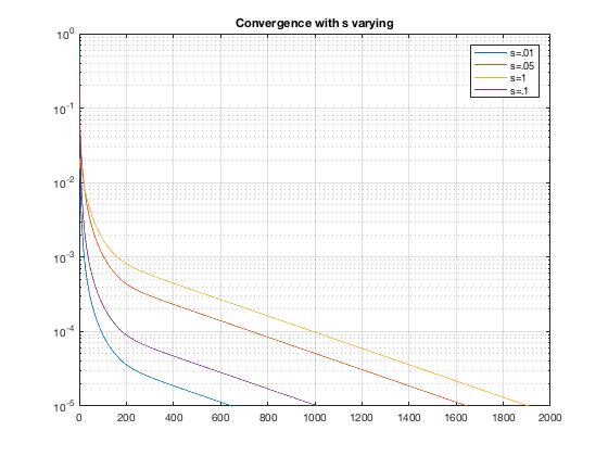
Instead of varying a parameter that affects the value of r, now we vary the value of sigma, which will affect the width of the gaussian distribution that is the initial condition. A larger value of sigma indicates a wider distribution. We see that when there is a narrower distribution, the solution takes longer to converge, but when the distribution is spread out wider, it will converge faster. This makes sense intuitively.