Linear Algebra Essentials: Part 2

December 20, 2020Themistoklis Haris

We conclude our chapter on the Adjoint of a linear operator.

Our main theorems

THEOREM:

Let $V$ be an inner product space and $T,U$ be linear operators on $V$ . Then:

$(T+U)^* = T^* + U^*$
$(cT)^* = \bar{c}T^*$
$(TU)^* = U^* T^*$
$(T^*)^* = T$
$I^* = I$

The proof of this theorem is based on the definition of the adjoint: $\langle T(x), y \rangle = \langle x, T^*(y) \rangle$ .

COROLLARY

The above properties hold for matrices too (through the $L_A$ operator)

APPLICATION: Least Squares Approximation

The definition of the problem is classic: Given $n$ points $(t_1, y_1), (t_2, y_2), . . . , (t_n, y_n)$ , we are trying to minimize $\sum\limits_{i=1}^n (y_i-ct_i-d)^2$ , with $c$ being the line of best-fit slope and $d$ is its offset. If

$A = \left [ \begin{array}{cc} t_1 & 1 \\ t_2 & 1 \\ . & .\\.&.\\.&.\\ \\ t_n & 1 \end{array} \right ], x = \left[\begin{array}{cc}c\\d\end{array}\right]$ and $y = \left[\begin{array}{cc}y_1\\y_2\\.\\.\\.\\y_n\end{array}\right]$

then we are basically trying to minimize $||y-Ax||^2$ . We will study a general method of solving this minimization problem when $A$ is an $m\times n$ matrix. This allows for fitting of general polynomials of degree $n-1$ as well. We assume that $m \geq n$ .

If we let $x \in \mathbb{R}^n$ and $y \in \mathbb{R}^m$ , then it is easy to see that $\langle Ax, y \rangle = \langle x, A^*y \rangle$ from the properties of the adjoint studied thus far. We also know that $rank(A^* A) = rank (A)$ by the dimension theorem, because the nullities of the two matrices are the same (this is straightforward to see). Thus, if $A$ has rank $n$ , then $A^* A$ is invertible.

Using these observations, our norm minimization problem can be solved through the minimality of orthogonal projections: Since $m \geq n$ , the range of $L_A$ is a subspace of $\mathbb{R}^n$ . The projection of $y \in \mathbb{R}^m$ onto $W$ is a vector $u = Ax_0$ and it is such that $||Ax_0 - y|| \leq ||Ax-y||$ for all $x \in \mathbb{R}^n$ . To find $x_0$ , let us note that $u-y$ lies in $W^{\perp}$ , so $\langle Ax, Ax_0 - y \rangle = 0$ for all $x \in \mathbb{R}^n$ . In other words, $\langle x, A^*(Ax_0 - y) \rangle = 0$ so $x_0$ solves the equation $A^* A x_0 = A^* y$ . If additionally the rank of $A$ is $n$ , we get that:

$x_0 = (A^*A)^{-1} A^* y$

APPLICATION: Minimal solutions to Systems of Linear Equations

How do we find minimal norm solutions to systems of linear equations? We prove the following theorem:

Theorem

Let $A \in M_{m \times n}(F), b \in F^m$ and suppose that the system $Ax=b$ is consistent. Then:

There exists exactly one minimal solution $s$ to $Ax=b$ and $s\in R(L_A^*)$ .
The vector $s$ is the only solution to $Ax=b$ that lines in $R(L_A^*)$ . So, if $u$ satisfies $(A A^*)u = b$ , then $s = A^* u$ .

In other words, finding minimal norm solutions to systems like $Ax=b$ can be done by finding any solution to the system $AA^* u = b$ and letting $x = A^* u$ .

Proof

The theorem follows relatively easily from the minimality of the projection onto a subspace (like before). We do, however, need that $N(L_A) = (R(L_A^*))^{\perp}$ , a fact which holds for all linear transformations. This fact can be easily established, so we leave it as an exercise.

Introduction to Spectral Graph Theory: Courant-Fischer Theorem

December 19, 2020December 19, 2020Themistoklis Haris

The following theorem gives a characterization of the eigenvalues of a symmetric matrix according to the Rayleigh quotient: the eigenvalues are the solution of a particular optimization problem

The Courant-Fischer Theorem

Let $M$ be a symmetric matrix with eigenvalues $\mu_1 \geq \mu_2 \geq \cdots \geq \mu_n$ . Then:

$\mu_k = \max\limits_{\substack{S\subset \mathbb{R}^n \\ dim(S) = k}} \min\limits_{\substack{x\in S \\ x\neq 0}} \frac{x^T M x}{x^T x}$ .

Proof

Step 1: Let $y_1, . . . , y_n$ be an orthonormal eigenbasis of $M$ , where $y_i$ belongs to the eigenspace of $\mu_i$ . Then we can write $x = \sum\limits_{i=1}^n c_i y_i$ , where $c_i = \langle y_i, x \rangle$ .
Step 2: We have that: $x^T M x = x^T M \left(\sum\limits_{i=1}^n c_i y_i\right) = x^T \left[\sum\limits_{i=1}^n c_i (M y_i) \right] = x^T \left (\sum\limits_{i=1}^n c_i \mu_i y_i\right) = \sum\limits_{i=1}^n c_i^2 \mu_i$ , as our basis is orthonormal.

Step 3: We prove that for some subspace $S$ of dimension $k$ we have that

$\min\limits_{\substack{x\in S \\ x\neq 0}} \frac{x^T M x}{x^T x} \geq \mu_k$ .

If we let $S = span(y_1, . . . , y_k)$ , then $x = \sum\limits_{i=1}^k c_i y_i$ and using our step 2, we get:

$\frac{x^T M x}{x^T x} = \frac{\sum\limits_{i=1}^k c_i^2 \mu_i}{\sum\limits_{i=1}^k c_i^2} \geq \frac{\sum\limits_{i=1}^k c_i^2 \mu_k}{\sum\limits_{i=1}^k c_i^2} = \mu_k$

Step 4: We prove that for all subspaces $S$ of dimension $k$ it is true that .

$\min\limits_{\substack{x\in S \\ x\neq 0}} \frac{x^T M x}{x^T x} \leq \mu_k$

We consider $T = span (y_k, . . . , y_n)$ of dimension $n-k+1$ . $S\cap T$ has dimension at least 1. So:

$\min\limits_{\substack{x\in S \\ x\neq 0}} \frac{x^T M x}{x^T x} \leq \min\limits_{\substack{x\in S\cap T\\ x\neq 0}} \frac{x^T M x}{x^T x} \leq \max\limits_{\substack{x\in T\\ x\neq 0}} \frac{x^T M x}{x^T x}$

Writing $x = \sum\limits_{i=1}^{k} c_i y_i$ for any $x \in T$ , we get that:

$\frac{x^T M x}{x^T x} = \frac{\sum\limits_{i=k}^n c_i^2 \mu_i}{\sum\limits_{i=k}^n c_i^2} \leq\frac{\sum\limits_{i=k}^n c_i^2 \mu_k}{\sum\limits_{i=k}^n c_i^2} = \mu_k$

From steps 3 and 4, our proof concludes.

Linear Algebra Essentials: PART 1

December 18, 2020December 19, 2020Themistoklis Haris

1. An introduction

Theorem 1

Let $V$ be an inner product space over $F$ and let $g\,:\,V\rightarrow F$ be a linear transformation. Then there exists a unique vector $y \in V$ such that $g(x) = \langle x,y \rangle$ for all $x \in V$ .

Definition

Let $T$ be a linear operator on an inner product space $V$ . The unique linear operator $T^*$ which is such that $\langle T(x), y\rangle = \langle x, T^*(y)\rangle$ is called the adjoint of $T$ .

Theorem 2

The adjoint of any linear operator exists.

Theorem 3

Let $V$ be a finite-dimensional inner product space, and let $\beta$ be an orthonormal basis for $V$ . Then $[T^*]_\beta = [T]_\beta^*$ .

Corollary: $L_{A^*} = (L_A)^*$

2. Proofs to the Theorems

PROOF OF THEOREM 1 (Every linear operator is an inner product operator)

Let $\beta=\{u_1,u_2, . . . ,u_n\}$ be a base for $V$ . Let A

$y = \sum\limits_{i=1}^n \overline{g(u_i)}u_i$ .

Then let $h(x) := \langle x,y\rangle$ . For $i \in [n]$ we have: $h(u_i) = \langle u_i, \sum\limits_{j=1}^n \overline{g(u_j)}u_j \rangle = \sum\limits_{j=1}^n g(u_j) \langle u_i, u_j \rangle = g(u_i)$ . Since $h$ and $g$ agree on every element of $\beta$ , they are equal linear operators. The uniqueness of $y$ follows easily through a contradiction argument.

PROOF OF THEOREM 2 (existence and uniqueness of the adjoint linear operator)

Let $y \in V$ . Define $g(x) = \langle T(x), y \rangle$ . It is easy to see that $g$ is linear. So, by Theorem 1, there exists a $y^* \in V$ such that $g(x) = \langle x, y^* \rangle$ . Defining $T^*(y) = y^*$ gives us the adjoint. Linearity and uniqueness follow easily.

PROOF OF THEOREM 3 (Adjoint representative is representative of conjugate transpose)

If $\beta=\{u_1,u_2, . . . ,u_n\}$ , then $([T^*]_\beta)_ij = \langle T^*(u_j), u_i \rangle = \overline{\langle T(u_i), u_j \rangle} = [T_\beta]^*$ .

2019: Looking back

December 31, 2019Themistoklis Haris

2019 was a fascinating year for me. I learned so many things and met so many people. I forged strong relationships and discovered a lot about myself. I worked hard and achieved many of my goals but also failed in many ways and realized how many things I need to improve on. I traveled around the world and I missed home. Thank God, I was healthy and my parents and friends were also healthy and I am grateful to be have been given opportunities to realize my dreams and pursue my interests.

The year is almost at an end. I am grateful to be able to spend these last 2 days in my home, with my parents. I will not work in this time. Instead, I will devote time to reflecting on the year that has passed and examine what I did, what I learned, where I can improve upon and what exactly I can change in the future.

How to fit one year into one post? Shall I examine 2019 chronologically? Or maybe categorically? I have decided to reflect in a categorical fashion. That is, I will first try to list out what I have learned academically, then I will look back on the relationships I have built, thus drawing some conclusions about what I have learned in a social setting and lastly I will try to look back on my travels and general experiences and see how my personality has changed in comparison to last year. I will not mention names or become overly specific about any information that doesn’t concern me.

1. Academics and work

I took a lot of very interesting classes this year, in Mathematics, Computer Science, Middle Eastern Studies and Russian Literature.

In Computer Science, I learned about:

- Generic Algorithms. The course covered topics from the famous CLRS book. Proofs of complexity and correctness were generally covered. Among the topics covered were:
  - Graph algorithms: Topological sort, Minimum Spanning Trees (Kruskal + Prim), SSSP and APSP, Maximum Flow.
  - Data Structures: Red-Black Trees, Heaps, Binary Indexed Trees, Segment Trees, Union-Find Disjoint Sets.
  - Algorithmic design: Dynamic Programming, Exhaustive Search and Greedy.
  - Complexity analysis: Expected running time, Average case running time, Amortized Complexity, Recursion solving
  - Sorting algorithms
  - String matching algorithms
  - Medians and order statistics
- Theory of Computation. A very fascinating topic. The course was particularly difficult, but offered me the chance to gain real mastery with the concepts presented. Among the topics covered were:
  - Finite Automata, Regular Expressions and Regular languages. Design of automata. Equivalence of deterministic and non-deterministic automata and regular expressions. Pumping lemma for regular languages.
  - Context-Free languages: push-down automata, context free grammars, pumping lemma, equivalence of PDAs and CFGs.
  - Turing Machines: mathematical definitions and properties.
  - Decidability, recognizability and unrecognizability of certain languages. Proofs by reduction.
  - Computational complexity theory: NP-completeness. Reduction proofs. 3-SAT and related problems. Cook-Levin Theorem. Computational Tableaux.
- Smartphone Programming in Android. Learning how Android APIs work in Java was quite interesting. There are a couple of concepts underlying the way an app works. Stuff like fragments, activities, XML and the UI, services, Google APIs like Firebase and Google Maps, Databases ans SQLite are all topics covered in the relevant course. I made an app called MyRuns, which was basically an activity tracker with GPS, database and cloud support and an app called NoChances, an antithesis to dating apps, whose function is to help people avoid each other!
- Machine Learning Basics. This course was definitely a great experience. I had a first experience of what everyone refers to as the current “trend” in Computer Science – data science. The way I see it, the task at hand is basically modeling the world not through precise equations as mathematicians do, but through existing instances of recorded facts. No one can take into account all possible factors that lead to a patient exhibiting some type of disease, but by considering millions of example cases and hundreds of measurable factors, we can statistically make assumptions with high accuracy. In the course, I learned about lots of classifiers, like Naive Bayes, Decision Trees, Support Vector Machines, Perceptrons, Logistic Regression and others. I also learned about clustering algorithms and a little bit about feature engineering.
- Compilers. I learned the basics of how compilers work. Going from lexical analysis to syntactic analysis with lex and yacc (byson) and then to an intermediate representations and optimizations (both global and local). Finally, I learned about code generation techniques and a little bit of Assembly. I actually built my own compiler for a small C-like language.
- Mixed Reality and 3D design. Through a research project, I investigated programming Mixed Reality interfaces. I experimented a lot both with hardware and software, learned the Unity platform and also investigated a bit how to make a simple server-client connection for an MR interface. Along the way, I picked up some 3d design skills in blender and Unity, realizing however how vast the field is and how much of an art it constitutes.
- Communication Complexity: As a research assistant, I learned the basis of a field in theoretical computer science that studies the efficiency of information exchange. I studied basic communication protocols, rectangle and rank methods of proving lower bounds for complexity, randomized protocols (public and private coin), distributional complexity and Yao’s lemma and the method of discrepancy. I also started investigating some properties of the Direct Sum problem and focused a bit on the disjointness function and its communication complexity properties.

In Mathematics, I learned about:

- Galois Theory and Field Theory: This branch of mathematics was really interesting and I can definitely say that I have not mastered it. Starting from field extensions, I learned about automorphisms, Galois extensions, Kummer extensions and the theory of polynomials. The class was particularly hard, but I learned a lot.
- Complex Analysis: Complex numbers are really powerful and have some fascinating properties. I learned about how we define differentiation and integration of complex-valued functions. I learned about properties of analytic functions, about the Cauchy Integral formula, Liouiville’s Theorem and the Maximum Modulus Principle. I also learned about complex series and about residues. Later, I also investigated the topic of analytic continuation.
- Other topics: I investigated by myself some other topics in mathematics, although I didn’t really dive in much depth. I looked into some number theory, with Riemann’s zeta function and into some information theory, with the basics of entropy. I also learned some basics of mathematical game theory.

I also learned a lot about Middle Eastern culture and history by taking the relevant introductory course at Dartmouth. I did research on Syria’s recent civil war and found out about some facts which I was largely ignorant of in the past.

Finally, I read some literature this year:

War and Peace, by Lev Tolstoy. I really enjoyed this book. Reading it took a lot of time, due to its sheer size. But the descriptions are stunning and the story is fascinating. The book also made me think about life philosophically in ways I hadn’t before. I took a class on Tolstoy’s literature, the professor for which I absolutely loved. She really helped me develop my passion for Tolstoy and take as much as I could from reading his works.
Crime and Punishment, by Fyodor Dostoyevsky. I haven’t finished that one yet. I am really liking it though.
Childhood, Boyhood, Youth, the first critically acclaimed work by Tolstoy in his 20s.
A lot of short stories by Tolstoy: Father Sergius, The Death of Ivan Ilych, Sevastopol Tales, Kroytzer Sonata, Master and Man

2. Social Matters

I have definitely built more relationships this year than any other year of my life. Initially, I think this can be attributed to a fervent desire within me to overcome a certain social insecurity: the constant desire of being needed. That feeling was consistently making me feel insufficient, and my seeking of social interactions was often, consciously of sub-consciously, aimed at extinguishing it. So I was living for myself. I was seeking friends to make myself feel needed. I recognized that selfishness within me and tried to move away from it.

I tried giving to people. I don’t have many things that people want from me, at least materially. I wouldn’t want to give in that sense either. But what I could give, I tried to give. I gave people time and attention. I gave them myself and I opened up and become more vulnerable. Many times this wasn’t appreciated and I was hurt. But many other times it was appreciated and I was really happy. I felt that giving unconditionally produced a happiness within me which I hadn’t felt before, at least intentionally.

However, I started to realize at some point that not everyone seeks to take from me. Deep inside me, I guess I was thinking of giving as a way to connect with everyone. Not being able to connect meant I just had to give more. But in building relationships with people, giving must necessarily be accompanied by at least some taking. One doesn’t demand nor expect to take, but mutual love necessitates some form of balance. Giving and taking also mustn’t be in the same form. Both people can contributed different things to keep the relationship alive. Their will to do so however, must be common and of relatively similar intensity. If only one person has a strong desire to cultivate the relationship and the other person does not, maybe the only way to guide the relationship to its natural state of equilibrium is for the one passionate giver to “back-off”. It is important to note here also, that “giving” and “taking” are very relative terms. One might, from their point of view, consider themselves as giving a lot, while the receiver might not even understand a tiny bit of what is being given to them, if any. Some agreement on these points of view is also necessary, at least in some subconscious level, for a relationship to blossom. But even a slight disagreement doesn’t ruin things. One thing that I have learned is that some things require effort to become effortless. Effort is usually good because it shows good intentions, but to stop trying is many times really hard and perhaps the best thing to do.

In total, I learned that it is important to have a balance and feel about giving in as much of an unconditional way as possible. One must not think about exchanges as a medium of feeling good only about themselves. People are interesting and beautiful and one can miss this beauty thinking only about their own self and image.

3. Traveling, Hobbies and Outlook on Life

I traveled around a lot this year. Let me list out all the places I went to, in chronological order:

Athens, Greece
Hanover, NH, USA
Boston, MA, USA
New Orleans, LA, USA -> LowerNine.org volunteer work
Montreal, Canada -> RGLP Immersion Experience
Athens, Greece -> Sounio! Beaches.
Florina, Greece
Hanover, NH, USA
(close to) Springfield, MA, USA -> Six Flags New England
San Jose, California, USA
Sunnyvale, California, USA -> Google!
Palo Alto, California, USA
San Fransisco, California, USA -> Fog. Didn’t see the bridge 🙁
Santa Clara, California, USA -> Swam in the pacific! Cold!
Hanover, NH, USA -> UGA Training. Camp Akeela.
Trips 2019! -> Trip leader! Hiking 2!
Boston, MA, USA -> Swim meet at Harvard
New York City, USA -> Columbia University, Ivy ISA Conference
Boston, MA, USA
Athens, Greece -> Driving lessons
Barcelona, Spain -> Sagrada Familia!
Granada, Spain -> Alhabra, tour of city!
Malaga, Spain -> Beautiful beach and castle
- Ronda, Spain -> Beautiful cliff and old city
Barcelona, Spain -> reached park guell. Closed because of wind 🙁
Athens, Greece
Thessaloniki, Greece -> Reunions 🙂 Harbors, swimming pool, city center
Florina, Greece
Patra, Greece -> Saw bridge of Rio-Antirrio! Quick stop for pizza
Athens, Greece -> War and Peace in theater.
Bansko, Bulgaria -> Snowboarding!
Athens, Greece -> Back home, reflecting on 2019!

Adding all the airports, I have been to this year, we get this map (I forgot Montreal):

I have taken up some new hobbies this year as well:

Go (Chinese board game)
Russian Literature
Snowboarding
Board games

As for my outlook on life, definitely a lot of things have changed this past year. I have learned some lessons which I will try to list below:

Live with love. This is the best way I can phrase it. I have learned that the most gratifying way to do things is with care and love. In every little thing we do, every little moment we live, we must live it with love. This is how work gains its best quality and how relationships gain the most meaning and authenticity.
Enjoy doubting. We must doubt everything we think we know. When we rest assured in knowledge we consider gained about life, we discover that there are countless other perspectives that may negate what we learned. There is no right answer or a single correct way to live. But there are always things to learn.
Live and let live. There are some things we cannot control. No matter how much I would like to sometimes, I cannot control how people act, what they think and what they do. That is something one needs to come to terms with.
Reflect critically.
Be compassionate and empathetic
Don’t take yourself (or anyone) too seriously .
Keep your eyes and ears open!
Don’t judge anyone (or yourself) too harshly.

So that’s my reflection on 2019! In about 3 hours, it will be 2020 and I will devote time to planning out a new decade! I’m sure it will be very different from the last. I will keep updating this post if I think of anything else that I can put on the list of things I can recall for 2019, but for now, that’s it!

Happy 2019!

Introduction to Direct Sums in Communication Complexity Theory

November 11, 2019September 7, 2020Themistoklis Haris

The direct sum problem concerns the following question: “If a task $A$ cannot be completed using less than $c$ steps, then do $k$ independent instances of task $A$ require at least $k\cdot c$ steps?”

In the theory of communication complexity, the task $A$ is calculating a certain function through some form of communication.

DEFINITION

Let $g\,:\,\{0,1\}^n\times\{0,1\}^n \rightarrow \{0,1\}$ be a function. We understand

$g^k\,:\,(\{0,1\}^n)^k\times(\{0,1\}^n)^k\rightarrow\{0,1\}^k$ ,

defined as:

$g^k((x_1, . . . ,x_k),(y_1, . . . ,y_k)) = (g(x_1,y_1), . . . ,g(x_k,y_k))$

to represent the task of performing $k$ different communications with the goal of calculating $g$ on $k$ different inputs.

QUESTION: Is $D(g^k) = kD(g)$ ?

An easy example of a relation $r$ for which a protocol exists that computes $r^k$ with less communication than $k$ times the minimum possible communication required to compute $r$ itself is the following:

Consider the following function: Let $n>0$ . Alice has a set $S\subset [n]$ of size $|S| = n/2$ . Bob has no input. The goal is Bob to produce an element of $S$ .

One strategy we can play with is Alice sending simply her smallest element to Bob. That requires $\left\lceil \log_2\left(\frac{n}{2} +1\right)\right\rceil$ bits, because the elements $\frac{n}{2}+2, . . . , n$ can never be the minimum of $S$ .

On the other hand, we require at least $\left\lceil \log_2\left(\frac{n}{2} +1\right)\right\rceil$ bits, because if a protocol existed that somehow made Bob aware of some element in $S$ using less than $\left\lceil \log_2\left(\frac{n}{2} +1\right)\right\rceil$ bits for any $S$ , then Bob would not be able to encode numbers outside of some set $P \subset [n]$ whose cardinality is at most $n/2$ . Thus, letting $S = [n] - P$ breaks the protocol.

So we need exactly $\left\lceil \log_2\left(\frac{n}{2} +1\right)\right\rceil$ bits to communicate some element of $S$ to Bob.

Now we shall show that we can have a protocol which, given any sequence $S_1, . . . , S_k \subset [n],\, |S_i| = n/2$ , can output a $k$ -tuple $(s_1, . . . , s_k)$ such that $s_i \in S_i\,\forall i \in [k]$ . The way that protocol works is the following:

We can prove that there exists a set $Q \subset [n]^k$ of $k$ -tuples $q = (q_1, . . . , q_k)$ with size $|Q| = nk2^k$ which is such that for any sequence $S_1, . . . , S_k \subset [n],\,|S_i| = n/2$ , there exists an element $q \in Q$ which is such that $q_i \in S_i\,\forall i \in [k]$ . Let us call this statement Lemma I and we will prove it below. Alice finds $Q$ exhaustively. Alice sends Bob the name of the element of $Q$ which works for the particular input. Overall, the cost of this communication is $k + \log_2(nk) \ll k\left\lceil \log_2\left(\frac{n}{2} +1\right)\right\rceil$ bits of communication.

PROOF OF LEMMA

We rely on the probabilistic method. We make $Q$ by repeating the following random experiment $nk2^k$ times: “Choose $n/2$ elements from $[n]$ by sampling each element uniformly at random.”

Given any sequence $S_1, . . . , S_k \subset [n], \,|S_i| = n/2$ , what is the probability that for all $q \in Q$ , there exists some $i \in [k]$ such that $q_i \notin S_i$ ?

The probability that for some given $q \in Q$ , we have that $q_i \in S_i$ for all $i \in [k]$ is $(\frac{1}{2})^{k}$ . Therefore, the probability that for some $q \in Q$ , at least some element misses its respective $S$ -set is $1 - (\frac{1}{2})^{k}$ . So the probability that this happens for all $q \in Q$ is

$(1- (\frac{1}{2})^{k})^{|Q|} \leq e^{-(\frac{1}{2})^k|Q|}$

So the probability that for all sequences $S_1, . . . , S_k$ , the $latex Q$ we constructed misses its mark is at most $2^{nk}e^{(1/2)^k|Q|} = 2^{nk}e^{-nk} < 1$ and so our proof concludes.

Next, we shall show that there is actually a lower bound to the deterministic communication cost $g^k$ , based on the fact that we can extract a monochromatic cover for $g$ through a monochromatic cover for $g^k$ .

THEOREM

If $g$ requires $c$ bits of communication, then $g^k$ requires at least $k(\sqrt{c}-\log n - 1)$ bits of communication.

PROOF

We will use the following Lemma II: “If the inputs to $g^k$ can be covered with $2^l$ monochromatic rectangles, then the inputs to $g$ can be covered with $\lceil 2n \cdot 2^{l/k}\rceil$ monochromatic rectangles.”

If we let $l$ be the communication cost for $g^k$ , then the inputs to $g^k$ can be covered by $2^l$ monochromatic rectangles and therefore, by the Lemma above, the inputs to $g$ can be covered by $\lceil 2n \cdot 2^{l/k}\rceil$ rectangles, implying (*) that the computing $g$ requires $c \leq \left(\frac{l}{k} + \log n + 1\right)^2$ bits communication, which finally yields that $l \geq k(\sqrt{c} - log n - 1)$ .

(*) This implication follows from a fundamental Theorem on rectangle covers, which we will not cover here for brevity, but in another post.

Now for the proof of Lemma II:

To produce a cover of $g$ with the necessary amount of rectangles, we show that given any $S \subseteq \{0,1\}^n \times \{0,1\}^n$ , there exists a rectangle $R$ that is monochromatic under $g$ and that covers at least $2^{-l/k}|S|$ of the inputs from $S$ . Applying this fact repeatedly $\lceil 2n\cdot 2^{l/k}/rceil$ times, we have left at most:

$2^{2n}\cdot \left(1-2^{-\frac{l}{k}}\right)^{2n\cdot 2^{l/k}} \leq 2^{2n}\cdot e^{-2^{-l/k}\cdot 2n2^{l/k}} = 2^{2n} \cdot e^{-2n} < 1$

elements which are uncovered and so our statement is proved.

For the proof of the key incremental claim, we exploit the fact that $(\{0,1\}^n)^k\times(\{0,1\}^n)^k$ can be covered by $2^l$ monochromatic rectangles, so that at least one “projection-rectangle” into the space $\{0,1\}^n\times \{0,1\}^n$ has a lot of elements.

Specifically, there must exist a rectangle $R'$ covering at least $2^{-l}|S|^k$ inputs from $S^k$ . Now, project $R'$ into its $i$ -th coordinate by retaining only the $i$ -th pair of inputs of Alice and Bob:

$R_i = \{(x,y) \in \{0,1\}^n\times \{0,1\}^n\,:\, \exists (a,b) \in R' \rightarrow a_i = x \wedge b_i = y\}$

$R_i$ is a rectangle because $R'$ is a rectangle, by invoking the basic rectangle-recognizability lemma and $R_i$ is also monochromatic under $g$ , since $R'$ is monochromatic under $g^k$ .

Now, we have that $R' = \prod\limits_{i=1}^{k}R_i$ , and so

$\prod\limits_{i=1}^{k}|R_i \cap S| \geq |R' \cap S| \geq 2^{-l}|S|$

Thus, for some $i \in [k]$ , we much have that $|R_i \cap S| \geq 2^{-l/k}|S|$ , which proves our claim and finishes our theorem.

A weak lower bound on the Communication Complexity of the Disjointness Function

October 25, 2019September 7, 2020Themistoklis Haris

Any private-coin randomized protocol $\pi$ that computes $DISJ_n$ with an error probability of at most $\epsilon$ cannot use less than some multiple of $\sqrt{n}$ bits in the worst case.

Invoke Newman’s Theorem

$R^{priv}_{\epsilon}(DISJ_n) = R^{pub}_{\epsilon-\delta} (DISJ_n) + O(\log n + \log \delta^{-1})$ .

Since $\sqrt{n} \gg \log n$ asymptotically, it suffices to show that

$R^{pub}_{\epsilon} (DISJ_n) = \Omega (\sqrt{n})$ , for $\epsilon \leq \frac{1}{3}$

Now recall Yao’s Lemma:

$R^{pub}_{\epsilon} (DISJ_n) \geq \max_{\mu}\{D^{\mu}_{\epsilon}(DISJ_n)$

which allows us to reduce the problem to coming up with a probability distribution $\mu$ over $X \times Y = \{0,1\}^n\times\{0,1\}^n$ such that any deterministic protocol which errs with probability of at most $\epsilon$ on any input according to $\mu$ communicates at least some multiple of $\sqrt{n}$ bits in the worst case.

One initial thought worth investigating is what happens when if $\mu =$ uniform. Suppose Alice and Bob both choose any subset of $[n]$ uniformly. Then the probability that they choose disjoint subsets is $\left(\frac{3}{4}\right)^n$ , which goes to 0 as $n$ grows large. So a protocol that just outputs 0 (they are NOT disjoint) can be made to have an arbitrarily small error asymptotically, which means that we only get an $\Omega(1)$ bound by using the uniform distribution. We are not satisfied.

Instead, consider the following product distribution: Alice and Bob cannot possibly pick a subset of $[n]$ whose size is different that $\sqrt{n}$ and they pick subsets of size $\sqrt{n}$ with uniform distribution. So $\mu = \lambda \times \rho$ , where:

$\lambda(X) = \rho(X) = \left\{ \begin{array}{ll} \!\! \frac{1}{\binom{n}{\sqrt{n}}}, &|X| = \sqrt{n}\\ \!\! 0, &\text{otherwise}\end{array}\right.$

In this case, the probability that Alice and Bob choose disjoint subsets is:

$\left(\frac{n-\sqrt{n}}{n}\right)^{\sqrt{n}} \approx \frac{1}{e}$

We will show that any deterministic protocol that, under $\mu$ , errs with a probability of at most $\epsilon$ in calculating $DISJ_n$ , uses at least some factor of $\sqrt{n}$ in the worst case.

The intuition is as follows: Let $\pi$ be the $(\epsilon-\mu)$ protocol with the minimum communication complexity. $\pi$ partitions $X\times Y$ into rectangles, corresponding to its leaves. For each rectangle, $\pi$ answers in the same way in the question of whether the two input subsets are disjoint or not.

However, some of these rectangles may be corrupted. In other words, the protocol may output that the input sets are disjoint, when in fact they are not. Let’s look at 1-rectangles. That is, rectangles in which the protocol answers YES, they are disjoint (1). We know that $\pi$ errs with a probability of at most $\epsilon$ . Therefore, all of its rectangles have small corruption. Specifically, if $R = S\times T$ is an 1-rectangle, then

$Pr_{\mu}\{DISJ(x,y)=0\,|,\, (x,y) \in R\} \leq \epsilon$

The figure below illustrates why that is.

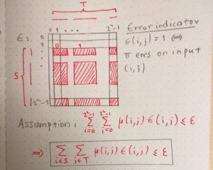
We show that exactly because the rectangles of $\pi$ cannot be too corrupted, they have to be small in size (their measure according to $\mu$ is small). This will imply that there are many of them and so we will have a lower bound to the communication complexity.

To elaborate further on this, let $A$ be the maximum $\mu$ -measure of any 1-rectangle of $\pi$ . If we suppose for the purposes of contradiction that $CC(\pi) \leq \alpha\sqrt{n}$ for some $\alpha$ , then the number of 1-rectangles is bounded above by the number of leaves of $\pi$ , which in turn is bounded above by $2^{\alpha\sqrt{n}}$ .

$1 = \sum\limits_{R}\mu(R) \leq 2^{\alpha\sqrt{n}}A$

And so $A \geq 2^{-\alpha\sqrt{N}}$ . In other words, if the communication complexity of $\pi$ is small, there must be a big 1-rectangle. And that rectangle has low corruption. We prove that this is impossible, acquiring a contradiction.

We prove the following Lemma (I):

“If $R=S\times T$ is a 1-rectangle of $\pi$ ,

then either $|T|$ or $|S|$ has to be at most $2^{-c\sqrt{n}}\binom{n}{\sqrt{n}}$ for some constant $c$ .”

After establishing this, if we let $R = S \times T$ be a 1-rectangle of $\pi$ and assume WLOG that $|T| \leq |S|$ , then $|T| \leq 2^{-c\sqrt{n}}\binom{n}{\sqrt{n}}$ by Lemma I, and so

$\mu(R) = \sum\limits_{s\in S, t\in T} \mu(s,t) = \left(\sum\limits_{s\in S}\lambda(s)\right)\left(\sum\limits_{t\in T} \rho(t)\right) \leq 1\cdot \frac{|T|}{\binom{n}{\sqrt{n}}} \leq 2^{-c\sqrt{n}}$ ,

which implies that every 1-rectangle $R$ must be small, thus giving us our contradiction.

Heading over to the proof of Lemma I, we first two simplifying assumptions:

S is large (we will formalize this below but if S were small then our lemma holds vacuously).
All the subsets of $[n]$ lying in $S$ and $T$ have size $\sqrt{n}$ . There is 0 probability of getting subsets of size $\neq \sqrt{n}$ as inputs, so Alice and Bob can modify $\pi$ to immediately reject such input cases so that we don’t have to worry about its behavior on them.

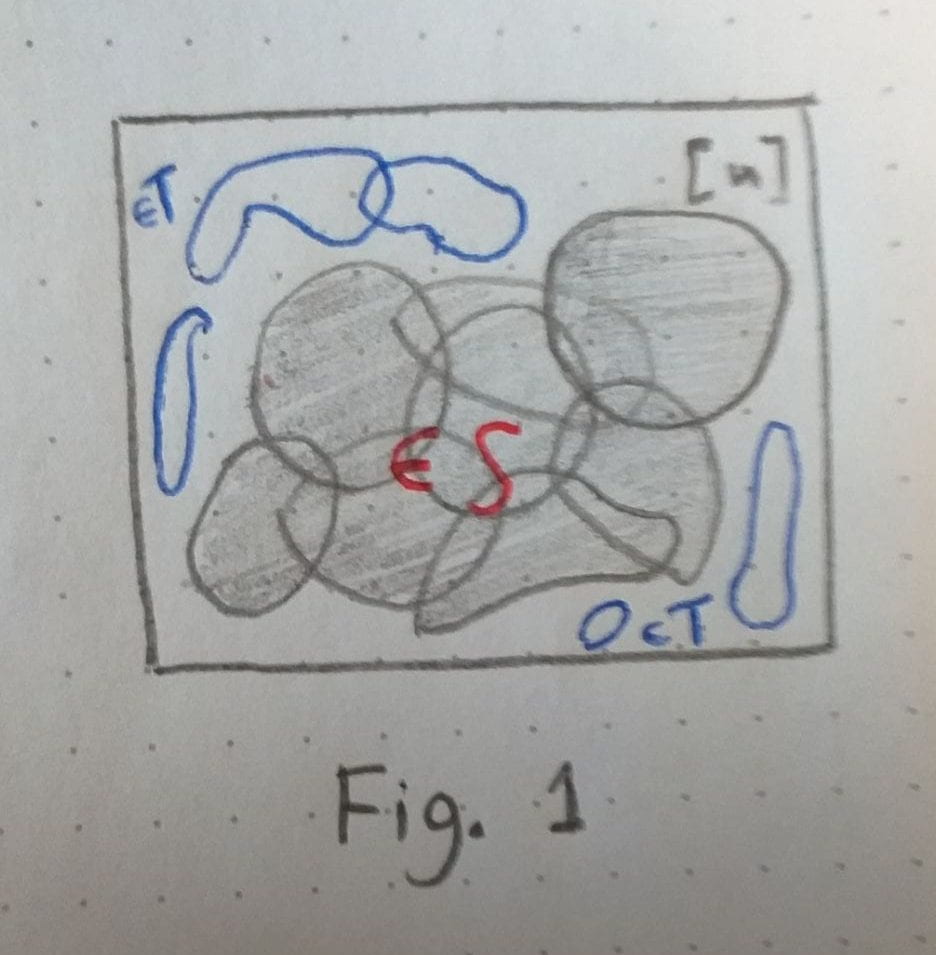
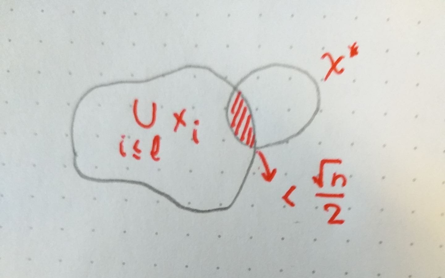
Intuition: If $S$ is large, then its sets must span a large fraction of $[n]$ . There cannot exist too many sets disjoint with the sets of $S$ then. So $T$ is small. This is illustrated in the figure below:

We shall start by proving that the span of the elements of $S$ has to be big. This is the following Lemma, which could be stated without any relation to our communication complexity investigations:

LEMMA II: Let $Q$ be a collection of subsets of size $\sqrt{n}$ of $[n]$ . Then there exists some $c'>0$ such that if $|Q| > \frac{1}{2} 2^{-c' \sqrt{n}} \binom{n}{\sqrt{n}}$ , then for $k = \frac{\sqrt{n}}{3}$ , there exist sets $x_1, x_2, . . ., x_k \in Q$ such that $\forall i=1,2, . . ., k$ it holds that

$\left|x_i \cap \bigcup\limits_{j<i}x_j \right| < \frac{\sqrt{n}}{2}$

Proof

We show that if we pick any $l < \frac{\sqrt{n}}{3}$ sets $x_1, x_2, . . ., x_l \in Q$ , we can find another set $x^{*} \in Q$ that shares less that $\frac{\sqrt{n}}{2}$ elements with the $l$ sets we picked.

In other words:

$\left|x^{*} \cap \bigcup\limits_{i\leq l} x_i\right| < \frac{\sqrt{n}}{2}$

This gives us an incremental procedure of finding the collection $x_1, x_2, . . ., x_k$ : Every new set we add has less than $\frac{\sqrt{n}}{2}$ common elements with all the previous sets chosen and this is exactly what we want to prove. This is shown in the figure below:

$|Z| = \left|\bigcup\limits_{i\leq l} x_i\right| \leq \sqrt{n}\cdot\frac{\sqrt{n}}{3} = \frac{n}{3} \Rightarrow |\{x \in Q\,:\, |x\cap Z| \geq \frac{\sqrt{n}}{2}| \leq$

$\leq \sum\limits_{i=\sqrt{n}/2}^{\sqrt{n}}\binom{n/3}{i}\binom{2n/3}{\sqrt{n}-i} \leq n\binom{n/3}{\sqrt{n}/2}\binom{2n/3}{\sqrt{n}/2} < 2^{-1-c'\sqrt{n}}\binom{n}{\sqrt{n}} < |Q|$

for large enough $n$ , where the constant $c'>0$ is obtained through Stirling’s approximation $\log_2 (n!) = n\log_2 n - n\log_2 e + O(log_2 n)$ . This concludes the proof of Lemma (II) because we have found that there must exist some $x^{*} \in Q$ such that $|x^{*} \cap Z| < \sqrt{n}/2$ .

Note that this Lemma implies that $Q$ spans a large portion of $U$ . Since each one of the $x_i$ -s adds at least another $\sqrt{n}/2$ new elements, we have that $|\cup_{x \in Q}| \geq \frac{\sqrt{n}}{3}\cdot \frac{\sqrt{n}}{2} = \frac{n}{6}$ , meaning that $Q$ spans at least one sixth of $U$ , which is a good fraction for our purposes.

Let’s now see exactly how $S$ having a large span forces $T$ to be small. The main idea lies in the fact that $R$ has low corruption, so we seek sets that are disjoint with most sets in $S$ and that number is bounded above because of the large span property.

Let $S'$ to be the set of elements in $S$ which are such that they intersect with a fraction of at most $2\epsilon$ of the sets of $T$ . We must have $|S'| \geq \frac{|S|}{2}$ , as if that wasn’t the case, there would be more than $\epsilon|S||T|\,$ $0$ s of $DISJ_n$ in $R$ and, because both $S$ and $T$ consist of rectangles of size $\sqrt{n}$ which we uniformly sample, that would violate our low-corruption hypothesis.

Applying Lemma II to $S'$ , we get that there exists some constant $c'>0$ such that if $|S'| > 2^{-1-c'\sqrt{n}}\binom{n}{\sqrt{n}}$ – implying the largeness of $S$ : $|S| > 2^{-c'\sqrt{n}}\binom{n}{\sqrt{n}}$ ) – then there exists a sub-collection $x_1, x_2, . . ., x_k$ of $S'$ with $k = \sqrt{n}/3$ whose span over $U$ is big as we saw before.

So let’s assume that $|S| > 2^{-c'\sqrt{n}}\binom{n}{\sqrt{n}}$ as dictated above and let us take $S'' = \{x_1,x_2, . . ., x_k\} \subset S'$ . Now also consider the sub-collection of $T$ consisting of sets that have an intersection with a fraction of at most $4\epsilon$ elements of $S''$ . Then $T'$ would have to contain at least half of the elements of $T$ – $|T'| \geq \frac{|T|}{2}$ – as otherwise there would be more than $2\epsilon|S''||T| \geq 2\epsilon |S'||T| \geq \epsilon|S||T|$ $0s$ in $R$ , contradicting once again our low-corruption hypothesis.

It is important to conceptually notice here how the low-corruption hypothesis forces large parts of $S$ and $T$ to not overlap with each other too much! So we seek sets that are mostly disjoint among the two groups. And the big span of $S$ constrains our options greatly. We show that there cannot be that many sets by bounding $T'$ from above.

For each set $y$ in $T'$ , there are at most $4\epsilon k$ sets in $S''$ which intersect it. So there must exist $k - 4\epsilon k = (1-4\epsilon)k$ sets $x_{i_1},x_{i_2}, . . , x_{i_{(1-4\epsilon)k}}$ in $S''$ that all don’t intersect it, which limits how many elements $y$ can possibly have. That is we must have that $y \subseteq [n] \setminus \cup_j x_{i_j}$ and knowing that each $x_{i_j}$ brings in at least $\sqrt{n}/2$ new elements, we must have $\left|[n] \setminus \cup_j x_{i_j}\right| \leq n - (1-4\epsilon)k\frac{\sqrt{n}}{2} \leq \frac{8n}{9}$ assuming that $\epsilon \leq 0.01$ . That doesn’t seem like a lot: all we said is that $y$ must be drawn from a fraction of $\frac{8}{9}$ -ths of the universe. But it provides us with the bound we needed.

The number of possible $y$ -s is at most:

$\binom{k}{(1-4\epsilon)k}\binom{8n/9}{\sqrt{n}} = \binom{\sqrt{n}/3}{4\epsilon\sqrt{n}/3}\binom{8n/9}{\sqrt{n}} < 2^{-1-c''\sqrt{n}}\binom{n}{\sqrt{n}}$ ,

where $c'' > 0$ is a constant given again by Stirling’s approximation.

So $|T| \leq 2|T'| < 2^{-c''\sqrt{n}}\binom{n}{\sqrt{n}}$ . Taking $c = min(c', c'')$ concludes our proof.

Riemann’s Rearrangement Theorem

August 11, 2019September 7, 2020Themistoklis Haris

This post will be devoted to a very special and surprising result given by the great Bernhard Riemann on the topic of the convergence of infinite series.

The theorem states:

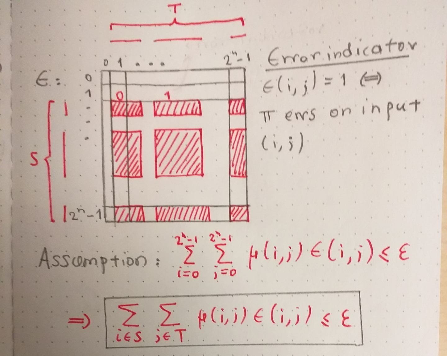
Let $\{a_n\}_{n=1}^{\infty}$ be a sequence of real numbers so that $\sum\limits_{n=1}^{\infty} a_n$ is conditionally convergent (it converges but not absolutely). Then if we let $M\in\mathbb{R}\cup\{\infty,-\infty\}$ , there exists a permutation $\sigma$ of $\{a_n\}$ such that $\sum\limits_{n=1}^{\infty} a_{\sigma(n)} = M$

Let’s let that result sink in first through a classic example. Consider the series $1 - \frac{1}{2} + \frac{1}{3} - \cdots = \sum\limits_{n=1}^{\infty}\frac{(-1)^{n+1}}{n}$ . We know this series converges to $ln(2)$ , through Taylor’s series but the series $\sum\limits_{n=1}^{\infty}\frac{1}{n}$ is the harmonic series and diverges. So our series is conditionally convergent. But observe that we can rearrange the terms of the infinite sum so that the series converges to the half of itself:

$\left(1-\frac{1}{2}-\frac{1}{4}\right) + \left(\frac{1}{3}-\frac{1}{6} - \frac{1}{8}\right) + \left(\frac{1}{5} - \frac{1}{10} - \frac{1}{12}\right) + \cdots = \sum\limits_{n=1}^{\infty}\left(\frac{1}{2n-1}-\frac{1}{4n-2} - \frac{1}{4n}\right) = \sum\limits_{n=1}^{\infty}\frac{1}{4k(2k-1)} = \frac{1}{2}ln(2)$

This is very weird. The same numbers added up in different order up to infinity, lead to a different sum. So addition works in strange ways when we take limits to infinity. We already sort of knew that but this theorem showcases it to an extent I couldn’t imagine before. And not only can we get half our sum by rearranging the terms, but we can get all possible numbers, by rearranging the terms in some way. We can even get $\pm \infty$ .

We should prove this important theorem. In fact we shall prove a stronger statement: that if $-\infty \leq a \leq b \leq \infty$ , there exists a rearrangement $\sigma$ of $\{a\}_{n=1}^{\infty}$ such that

$\liminf_{n\rightarrow\infty}s_n'= a$ and $\limsup_{n\rightarrow \infty}s_n' = b$ ,

where $s_n'$ is the sequence of partial sums of the rearranged sequence.

We get our result immediately if $a=b$ . In case there is confusion about the $\limsup$ and $\liminf$ notation, recall that these signify the limit superior and limit inferior of a sequence, which are limiting bounds on a sequence (more info here).

First, define the following sequences: $p_n = \frac{|a_n| + a_n}{2}$ and $q_n = \frac{|a_n|-a_n}{2}$ . So $p$ consists of all the positive terms in $a$ and of 0s in the place of the negative terms and $q$ is the opposite.

FACT: $p$ and $q$ diverge.

This isn’t very hard to see. If they both converged then $\sum|a_n|$ would have to converge and if one converged and one diverged then $\sum a_n$ would converge (check this!)

Now consider the sequences $P_n, Q_n$ of positive terms and of the absolute values of the negative terms in order in $\sum a_n$ . P and Q differ from p and q only in the placement of 0s in between of the latters’ terms, so both P and Q diverge.

IDEA / GOAL: Construct sequences $\{m_n\}, \{k_n\}$ such that the series

$P_1 + \cdots P_{m_1} - Q_1 -\cdots - Q_{k_1} + \\[1mm] P_{m_1+1} + \cdots + P_{m_2} - Q_{k_1+1} - \cdots - Q_{k_2} + \cdots$

,which is obviously a rearrangement of $\sum a_n$ satisfy our theorem’s target.

How to do this? First choose sequences $\alpha_n \rightarrow a, \beta_n \rightarrow b$ so that $\beta_1 > 0$ and $\alpha_n < \beta_n$ . Then let $m_n$ and $k_n$ be the smallest integers such that

$x_n = \sum\limits_{i=0}^{m_n}P_i - \sum\limits_{i=0}^{k_{n-1}} Q_i > \beta_n$ and $y_n = \sum\limits_{i=0}^{m_n}P_i - \sum\limits_{i=0}^{k_n} Q_i < \alpha_n$ (let $k_0 = -1$ )

We can always find such integers because $P, Q$ diverge.

Since $m_n$ and $k_n$ are the smallest integers with this property, we have that $|x_n - \beta_n| \leq P_{m_n}$ and $|y_n - \alpha_n| \leq Q_{k_n}$ so that $x_n \rightarrow a$ and $y_n \rightarrow b$ .

Finally, it is clear that no subsequential limit of our rearranged series can converge to something larger than b or smaller than a and so our proof is complete.

Proof adapted from the book “Principles of Mathematical Analysis”, by Walter Rudin.

2D Max Sum of Subarray – Kadane’s algorithm

August 6, 2019September 7, 2020Themistoklis Haris

Consider a matrix M $m\times n$ with integer values. We seek to find a rectangular subarray of M whose sum of elements is maximized.

$\begin{matrix} 5 & -4 & -3 & 4 \\ -3 & -4 & 4 & 5 \\ 5 & 1 & 5 & -4 \end{matrix}$

First, let’s examine the 1D version of the problem. The brute force approach would be $O(n^2)$ as we would have to examine all subarrays of M and build up the sums incrementally. A cleverer way is by using Dynamic Programming in Kadane’s algorithm.

Let $P(i)$ denote the maximum sum subarray of M ending at index $i$ . We can easily see how the following recursive formula holds:

$P(i) = \left\{ \begin{array}{ll} M[i], &\text{if } i=0 \\ \max\{M[i], M[i]+P(i-1)\}, & \text{otherwise} \end{array} \right.$

After finding $P(i)$ for all i, we can loop through those values to get the maximum one. The time complexity is $O(n)$ .

For the 2D version of the problem, we employ a small trick. We examine the space between all possible pairs of columns. Let $c_1$ and $c_2 \geq c_1$ be two columns of M. Then we want to constructively construct an array T such that T[i] holds the sum of all values of row i of M between the two columns. On T we run Kadane’s algorithm for 1D to get our solution. This algorithm runs in $O(n^3)$ over the $O(n^4)$ brute force approach.

Animation, 3D Rigging, Mixed Reality and more Unity

August 2, 2019September 7, 2020Themistoklis Haris

In recent weeks, I have been working a lot to augment my MR project for my research through modifying the animation tracks present in it. I will record many of my conclusions, progress and understanding in this page.

Firstly, I was briefly exposed to the vast field of Computer Animation. I was in possession of a Humanoid Avatar, which was rigged and animated according to some motion capture data. I first had to understand some of the mechanics of Unity’s animation system, which was recently changed relative to the past. In Unity, to animate a GameObject, one must first attach an Animator component to it. The Animator component contains an Animator Controller. This Controller is a whole different beast altogether and can be wired up using the special Animator window. In short, it contains multiple Layers, which one can animate and each layer contains a State Machine which ties into how something is animated. Each state contains an Animation Clip, which can either be composed in Unity’s animation window or be some external thing.

Animation Clips can be produced through the animation window through pose rigging. One simply rigs a couple of poses in succession to one another and then Unity interpolates through them to produce the clip. Of course, there are a lot to see and do at this stage. One can control the interpolation curves to make the animation smoother or more cartoonish. And of course one can control the speed of the animation, make it loop etc… All those elements of animation in Unity are accessible through code in C#, where I found that pausing / continuing an animation is possible simply by tweeking its speed. This is also required in other cases too, like when most animation clips are too fast.

As a final part to experiencing Unity’s animation environment, I also played around with the Timeline, a tool that allows the user to play animations and activate / deactivate objects in succession. This allowed me to build quite a cool little application in MR and would have made things extremely easy if I was aware of its existence early on, because in the beginning I would devote hours to synchronizing different Animators manually, while this tool does it better and automatically.

In terms of MR, I practiced a lot linking the controllers to code and giving the user control over their Mixed Reality experience. I implemented an application in which the user can rotate, shrink and transport humanoid avatars with their controllers while they are performing some animation clip. The user could also pause / continue that animation.

For the humanoid avatars, I spent quite a bit of time thinking and experimenting with different models. I first chose a very rudimentary model from the Unity Asset Store and then upgraded it to the “Man In A Suit” model. Lastly, I started using UMA 2 (Unity Multipurpose Avatar), which is very customizable and well-rigged but was kind of buggy and gave me trouble more than once. I realized that using the Bone Builder tool is the way to go to achieve integration of UMA in the Timeline. Important fact: UMA AVATARS NEED A FLOOR underneath them or they will fall to infinity because they are by default rigidBody objects (I just realized this).

And speaking of floors, I also spent a lot of time thinking about how to make this floor invisible, because I certainly didn’t want it to show up in my MR application. The solution I used in the end was something called a stencil shader. A stencil shader is a type of shader that is used to hide parts of a mesh for being shown in the screen. I will compile my efforts to understand more about shaders in another post.

Lastly, I also had to synthesize one my own animation clips of a rigged hands model. Producing this kind of animation is something that may be doable through Unity but I used Blender to do it. Again, I had to rig each pose individually and it was quite time consuming, but I got to see how Blender works and a bit of its mechanics.

VR/MR/AR, C# and Unity – DAY 7

July 11, 2019September 7, 2020Themistoklis Haris

Picking up from where I left off last time, my problem today is mainly hardware related. I cannot get the VivePro and Zed to agree in Unity and so the display is just black!

The solution which I found was using ZED_Rig_Stereo, instead of ZED_Rig_Mono (later confirmed by staff in StereoLabs), because the latter simply uses just the left camera, while the headset needs input from both cameras to function. But then my problem was immense glitching and jumping in the image!

I tried so many things: installing new NVIDIA drivers, changing GPU settings, clearing up memory in the disk etc… But nothing really worked. And I also had problems with the Vive not connecting easily.

With the help of a staff member at StereoLabs, I finally reached a working solution: disable tracking in the ZEDManager. That means that all the tracking info which the Zed uses come from the VivePro, whose tracking is actually much better, given that it has two points of reference (base-stations). But my VivePro has been having a lot of difficulties tracking. So, after looking online at forums of people with similar problems, I got the idea that maybe the windows, which I opened to let more light in for the sake of the Zed, actually reflect the lasers emitted from the base stations and prevent tracking. Truly, as soon as I shut the blinds, tracking with the VivePro became easier again and I could produce a working demo of my code.

Success!

Plans for the week to come:

Ensure that the ZED+VivePro is working smoothly and pinpoint conditions in different environments which cause problems or that work particularly well.
Attach the 3D printed mount on the VivePro in a stable way.
Run the 3D avatar on VR and then on MR and customize it so that it provides a good teaching experience. Also add some textual instructions around it.
Research how you can infer the relative position of the hands through the ZED.